Canonical Components

Open in Colab

Canonical covariance analysis (aka partial least squares correlation) finds linear relationships between pairs of datasets that have the same number of data points but usually have different numbers of features. It specifically finds k pairs of coefficient vectors that transform the original data points into k pairs of components, in a way that maximizes the total covariance over all pairs of components.

This method is popular across diverse scientific fields, but its application to data with many features can often lead to unstable estimates of coefficients. This problem can be ameliorated, to some extent, through the adoption of sparse variants of these methods.

Here, we extend the Loyvain method to do sparse binary canonical covariance analysis. We illustrate this method for finding the cross-correlation structure of structural and correlation networks from our example brain-imaging data.

Set up and load data

# Install abct and download abct_utils.py
base = "https://github.com/mikarubi/abct/raw/refs/heads/main"
!wget --no-clobber {base}/docs-code/examples/abct_utils.py
%pip install --quiet abct nilearn

# Import modules
import abct
import numpy as np
from abct_utils import W, C, fig_scatter, fig_surf

File ‘abct_utils.py’ already there; not retrieving.

Note: you may need to restart the kernel to use updated packages.

Run canonical covariance analysis

A common formulation of canonical covariance analysis centers on the detection of (principal) components of cross-covariance matrices. We build on this formulation to extend the Loyvain algorithm to do a binary variant of this analysis by independently clustering the rows and columns of cross-covariance matrices, or any other bipartite (two-part) networks, for that matter. This process simultaneously finds pairs of modules from both datasets and is equivalent to canonical covariance analysis with binary coefficients.

# Number of canonical components
k = 5

# Weighted canonical covariance analysis (with degree correction by default)
np.random.seed(1)
A_wei, B_wei, U_wei, V_wei, R_wei = abct.canoncov(W, C, k, "weighted")

# Reverse the signs of the coefficients
# (signs of canonical coefficients are arbitrary)
A_wei = - A_wei
B_wei = - B_wei
U_wei = - U_wei
V_wei = - V_wei

# Binary canonical covariance analysis (with degree correction by default)
A_bin, B_bin, U_bin, V_bin, R_bin = abct.canoncov(W, C, k, "binary")

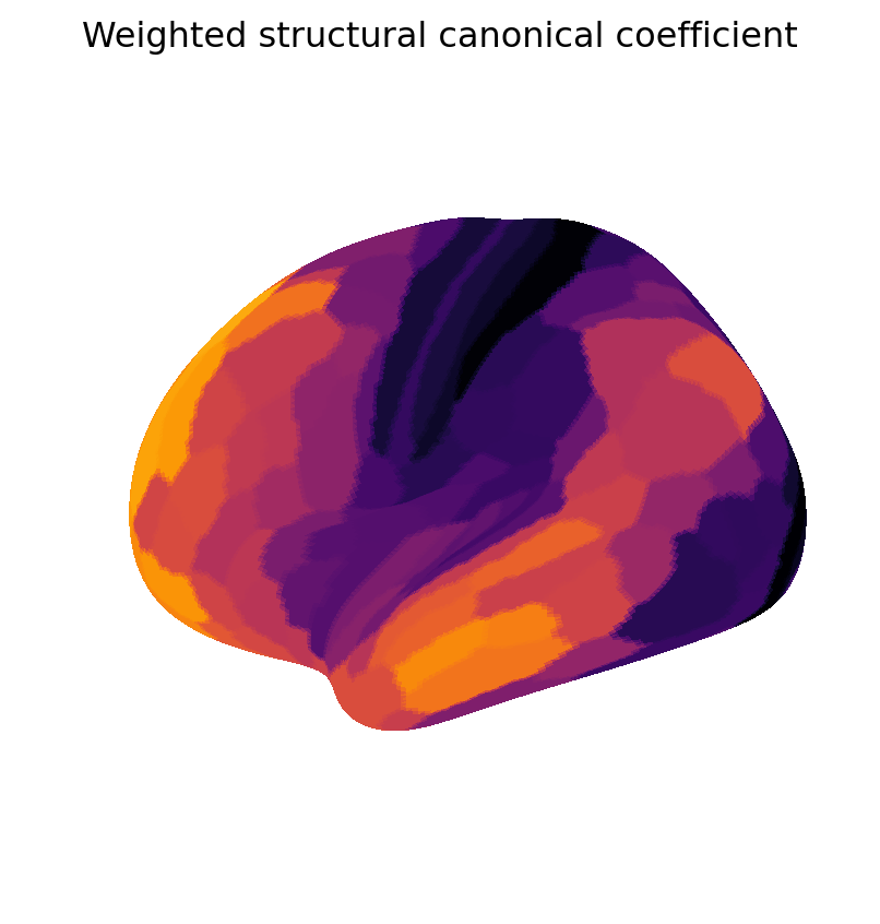
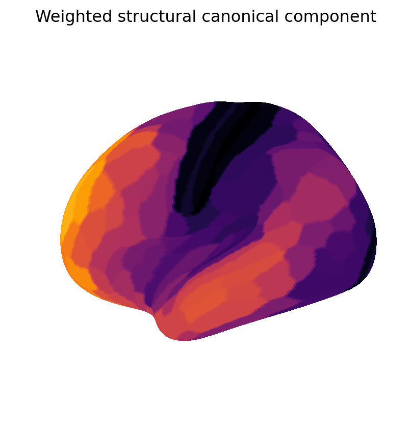
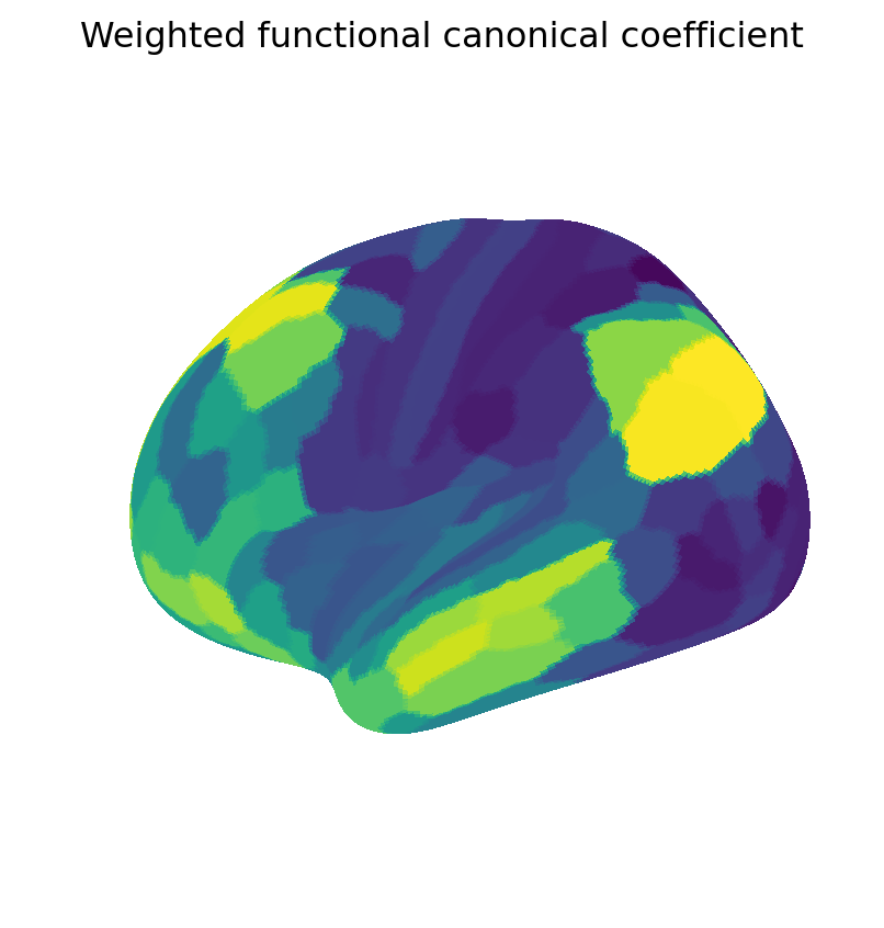
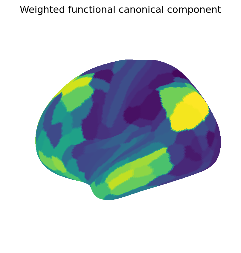
Show maps of weighted and binary canonical coefficients and components

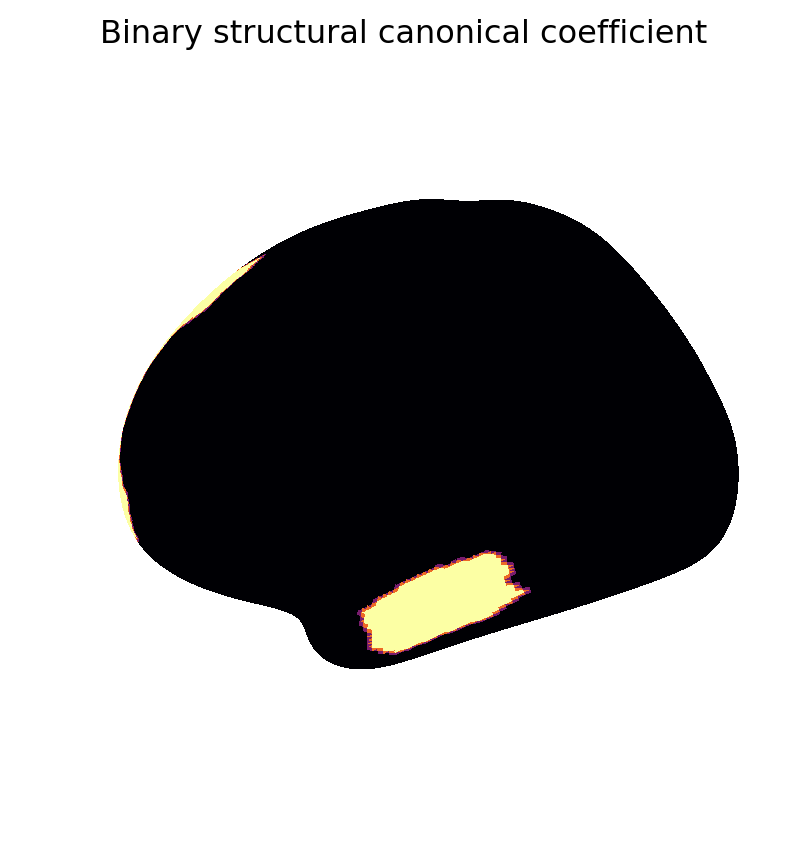
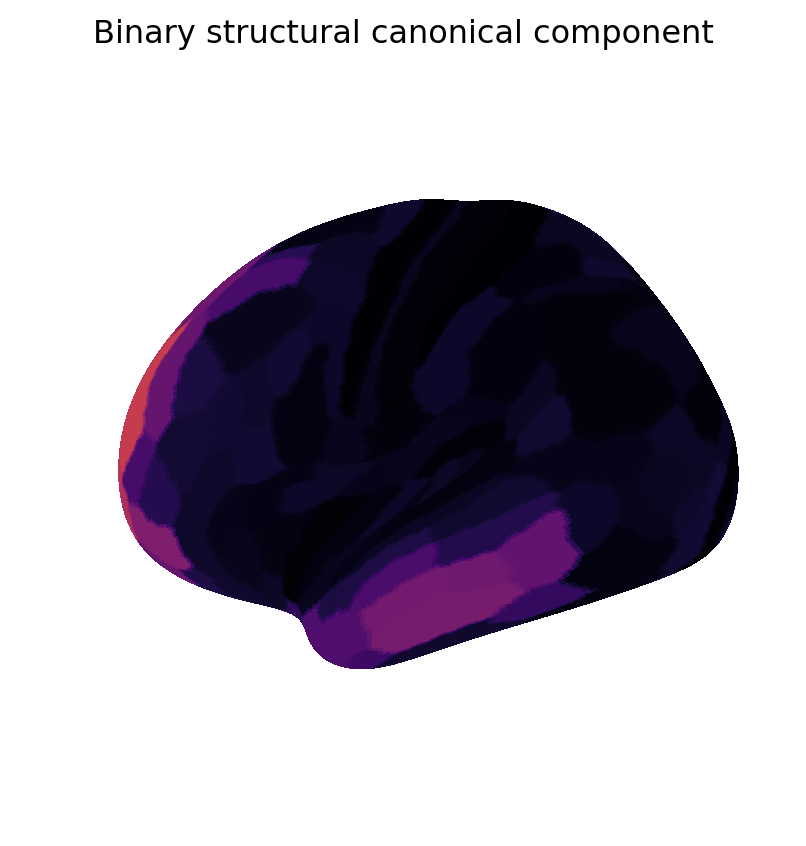
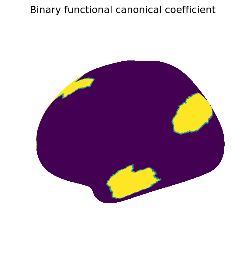
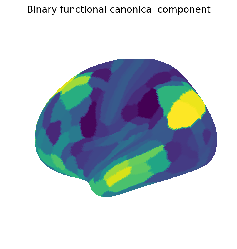
We now visualize maps of the weighted and binary canonical coefficients and components. These results show that binary coefficients can be sparse and more interpretable than their weighted counterparts. Moreover, binary coefficients lead to a particularly simple definition of canonical components, as sums of data points over the non-zero features.

ccas = {"Weighted structural canonical coefficient": (A_wei[:, 0], "inferno"),
        "Weighted structural canonical component": (U_wei[:, 0], "inferno"),
        "Weighted functional canonical coefficient": (B_wei[:, 0], "viridis"),
        "Weighted functional canonical component": (V_wei[:, 0], "viridis"),
        "Binary structural canonical coefficient": (A_bin[:, 0], "inferno"),
        "Binary structural canonical component": (U_bin[:, 0], "inferno"),
        "Binary functional canonical coefficient": (B_bin[:, 0], "viridis"),
        "Binary functional canonical component": (V_bin[:, 0], "viridis")}

for i, (name, vals_cmap) in enumerate(ccas.items()):
    vals, cmap = vals_cmap
    fig_surf(vals, name, cmap)

Visualize scatters of canonical covariances

We now visualize the normalized covariances between the first five canonical components from the weighted and binary canonical covariance analyses. Note that the values of these covariances are not directly comparable due to different normalizations of the weighted and binary analyses.

fig_scatter(np.arange(k), R_wei, 
            "Canonical components", 
            "Canonical covariances", 
            "Weighted canonical covariance analysis").show()

fig_scatter(np.arange(k), R_bin, 
            "Canonical components", 
            "Canonical covariances", 
            "Binary canonical covariance analysis").show()

Visualize scatters of canonical components

Finally, we directly show the relationship between the first weighted and binary canonical components. These results show generally high correlations between these components. We note, however, that these high correlations are not necessarily guaranteed because binary constraints can, in principle, result in considerably different components.

# Scatter plot of structural canonical components
rs = np.corrcoef(U_wei[:, 0], U_bin[:, 0])[0, 1]
fig_scatter(U_wei[:, 0], U_bin[:, 0],
            "Weighted canonical components",
            "Binary canonical components",
           f"Structural canon. comp. (r = {rs:.3f})").show()

rf = np.corrcoef(V_wei[:, 0], V_bin[:, 0])[0, 1]
fig_scatter(V_wei[:, 0], V_bin[:, 0],
            "Weighted canonical components",
            "Binary canonical components",
           f"Correlation canon. comp. (r = {rf:.3f})").show()