Degree Centralities

Open in Colab

Degree is a basic measure of node centrality, defined as the sum of node connection weights. Here, we show the equivalence of the degree and its extension, the second degree, with five measures of communication, control, and diversity. Since many of these measures assume that activity propagates on physical networks, we primarily study them on structural networks in our example brain-imaging data.

Set up and load data

# Install abct and download abct_utils.py
base = "https://github.com/mikarubi/abct/raw/refs/heads/main"
!wget --no-clobber {base}/docs-code/examples/abct_utils.py
%pip install --quiet abct nilearn nctpy bctpy

# Import modules
import abct
import numpy as np
from scipy import sparse
from nctpy import utils, metrics
from bct import mean_first_passage_time
from abct_utils import W, fig_scatter, fig_surf

File ‘abct_utils.py’ already there; not retrieving.

Note: you may need to restart the kernel to use updated packages.

Relationship between degree and measures of diffusion

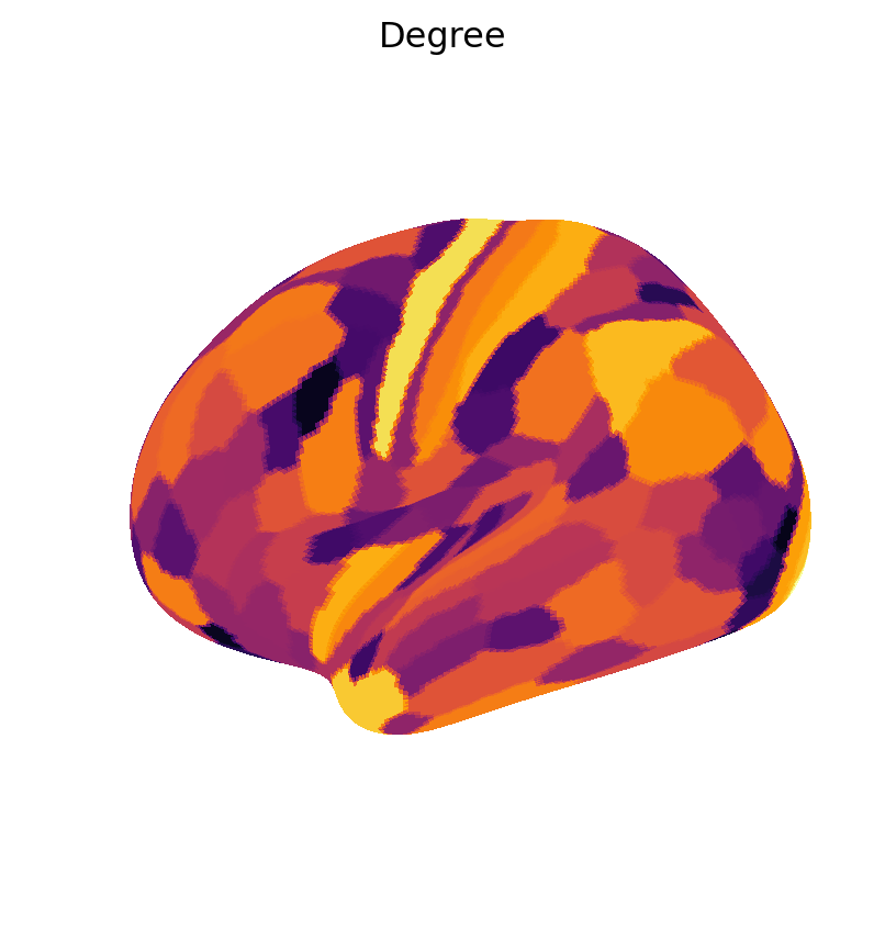
We first consider the weighted degree (or strength), defined for each node as the sum of its connection weights. We compute and visualize the map of the degree.

Degree = abct.degree(W, "first")
fig_surf(Degree, "Degree", "inferno").show()

/tmp/ipykernel_300480/2920194165.py:2: UserWarning:

FigureCanvasAgg is non-interactive, and thus cannot be shown

In many cases of interest, the degree is approximately equivalent to eigenvector centrality and diffusion efficiency, two popular measures of nodal centrality based on the assumption of diffusion dynamics or random walks.

Eigenvector_centrality = sparse.linalg.eigs(W, k=1)[1].real.ravel()
Eigenvector_centrality *= np.sign(np.sum(Eigenvector_centrality * Degree))

Diffusion_efficiency = 1/mean_first_passage_time(W).mean(0)

r = np.corrcoef(Degree, Eigenvector_centrality)[0, 1]
fig = fig_scatter(Degree, Eigenvector_centrality, 
                 "Degree", 
                 "Eigenvector centrality", 
                f"Structural network (r = {r:.3f})").show()

r = np.corrcoef(Degree, Diffusion_efficiency)[0, 1]
fig = fig_scatter(Degree, Diffusion_efficiency, 
                 "Degree", 
                 "Diffusion efficiency", 
                f"Structural network (r = {r:.3f})").show()

Relationship between second degree and measures of communication and control

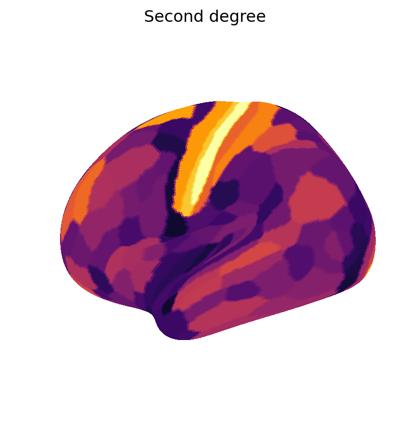
We next consider the second degree, defined for each node as the sum of its squared connection weights. We compute and visualize the map of the second degree.

Second_degree = abct.degree(W, "second")
fig_surf(Second_degree,
        "Second degree",
        "inferno").show()

/tmp/ipykernel_300480/1759232829.py:4: UserWarning:

FigureCanvasAgg is non-interactive, and thus cannot be shown

The second degree is exactly or approximately equivalent to communicability centrality, average controllability, and modal controllability, three popular measures of communication and control. These measures are also based on the assumption of diffusion dynamics and consider the number and length of all possible walks between two pairs of nodes.

# Normalize for communicability analysis
W_nrm1 = W / sparse.linalg.eigs(W, k=1)[0].real
Communicability = np.diag(sparse.linalg.expm(W_nrm1))

# Normalize for controllability analysis
W_nrm2 = utils.matrix_normalization(W_nrm1, "discrete")
Ave_control = metrics.ave_control(W_nrm2, "discrete")
Mod_control = metrics.modal_control(W_nrm2)

r = np.corrcoef(Second_degree, Communicability)[0, 1]
fig = fig_scatter(Second_degree, Communicability, 
                 "Second degree", 
                 "Communicability", 
                f"Structural network (r = {r:.3f})").show()

r = np.corrcoef(Second_degree, Ave_control)[0, 1]
fig = fig_scatter(Second_degree, Ave_control, 
                 "Second degree", 
                 "Average controllability", 
                f"Structural network (r = {r:.3f})").show()

r = np.corrcoef(Second_degree, Mod_control)[0, 1]
fig = fig_scatter(Second_degree, Mod_control, 
                 "Second degree", 
                 "Modal controllability", 
                f"Structural network (r = {r:.3f})").show()