Co-neighbor Components and Residual Degree

Open in Colab

Diffusion-map embedding is a versatile method for nonlinear dimensionality reduction. One variant of this method has transformed analyses in much of imaging neuroscience by robustly detecting co-activity (functional) gradients, low-dimensional representations of correlation networks that capture important properties of functional organization.

Here, we show an approximate equivalence between the components of co-neighbor networks — a simple class of integer networks — and this variant of diffusion-map embedding in our example brain-imaging data.

Set up and load data

# Install abct and download abct_utils.py
base = "https://github.com/mikarubi/abct/raw/refs/heads/main"
!wget --no-clobber {base}/docs-code/examples/abct_utils.py
%pip install --quiet abct nilearn

# Import modules
import abct
import numpy as np
from abct_utils import W, C, ordc, fig_scatter, fig_surf, fig_imshow

File ‘abct_utils.py’ already there; not retrieving.

Note: you may need to restart the kernel to use updated packages.

Visualize co-neighbor networks

Co-neighbor networks, as their name suggests, encode the number of shared 𝜅-nearest, or strongest correlated, neighbors between pairs of nodes. We first visualize the structure of co-neighbor correlation networks in our data.

# Define and visualize co-neighbor networks
# (kappa = 0.1 is equivalent to the top 10% nearest neighbors)
Cn = abct.kneighbor(C, "common", 0.1).toarray()

fig_imshow(Cn[np.ix_(ordc, ordc)],
           "Correlation co-neighbor network",
           "viridis").show()

Get co-activity gradients

Next, we compute the components of co-neighbor networks.

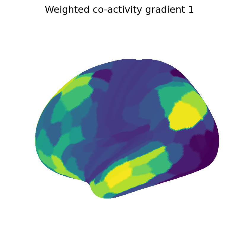
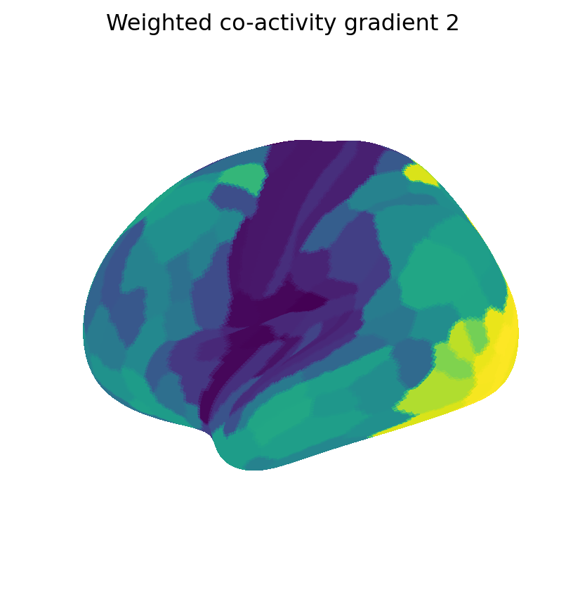
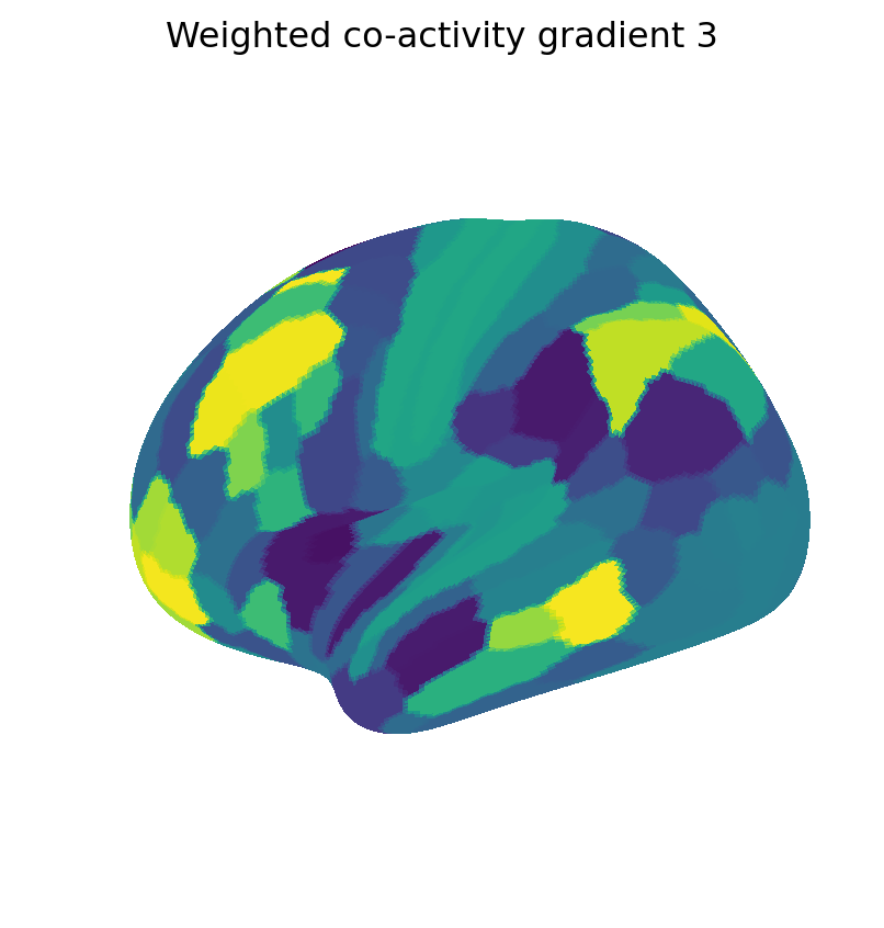
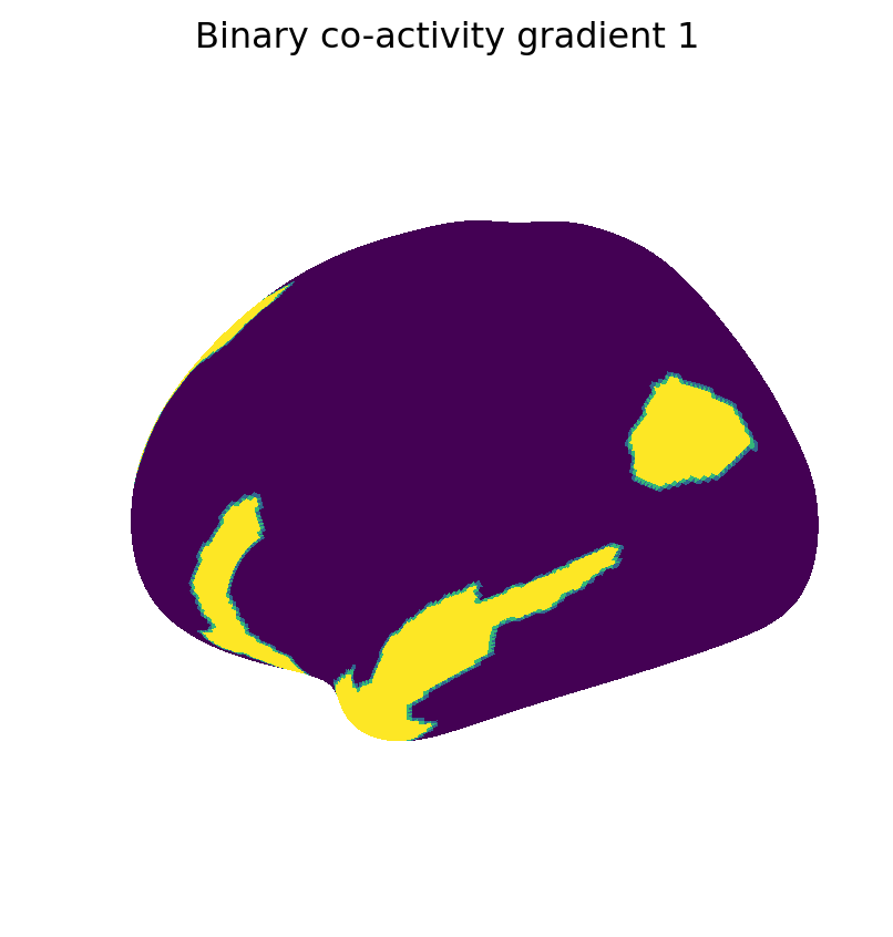
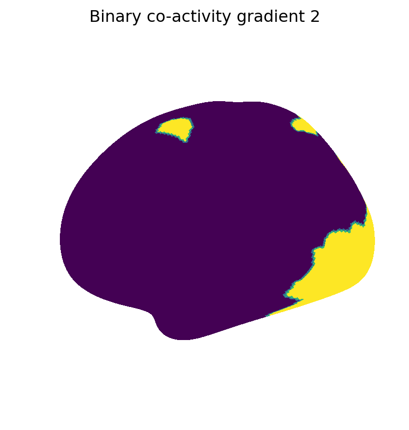
np.random.seed(1)

# Define co-activity gradient parameters (see kneighbor)
k = 5
kwargs = {"type":"common", "kappa":0.1, "similarity":"network"}

# Weighted co-activity gradients
V_wei = abct.kneicomp(C, k, "weighted", **kwargs)
V_wei = V_wei[:, [0, 1, 3]] # match components to standard order

# Binary co-activity gradients
V_bin = abct.kneicomp(C, k, "binary", **kwargs)
V_bin = V_bin[:, [1, 2, 3]] # match components to standard order

# Flip sign of weighted gradients to match binary gradients
V_wei *= np.sign(np.sum(V_wei * V_bin, 0))

Show maps of weighted and binary co-activity components

We now show the maps of three weighted and binary co-activity components. These maps closely resemble the maps of co-activity gradients estimated with diffusion-map embedding.

comps = {"Weighted co-activity gradient": (V_wei, "viridis"),
        "Binary co-activity gradient": (V_bin, "viridis")}

for i, (name, Vals_cmap) in enumerate(comps.items()):
    Vals, cmap = Vals_cmap
    for j in range(Vals.shape[1]):
        fig_surf(Vals[:, j], f"{name} {j+1}", cmap)

Show map and scatter of residual degree

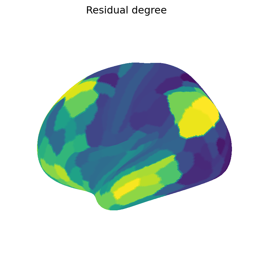
The primary co-activity gradient plays an especially important role in imaging neuroscience because it represents a transition between primary and association cortical areas. We conclude by showing a particular simple approximation of this component, as the degree of the residual network after first-component removal, or global signal regression.

# Residual degree
D_wei = abct.degree(C, "residual")

# Map of residual degree
fig_surf(D_wei, "Residual degree", "viridis")

# Scatter of residual degree and weighted co-activity gradient
r = np.corrcoef(D_wei, V_wei[:, 0])[0, 1]
fig = fig_scatter(D_wei, V_wei[:, 0], 
                 "Residual degree", 
                 "Weighted co-activity gradient", 
                f"Correlation network (r = {r:.3f})").show()