UMAP is a prominent manifold-learning method especially popular in the analysis and visualization of single-cell, population-genetic, and other biological data. Here, we consider the performance of the first-order approximation of (the true parametric) UMAP objective on our example brain-imaging data. We term this approximation m-umap, and note that it reduces to a generalized modularity.
File ‘abct_utils.py’ already there; not retrieving.

Note: you may need to restart the kernel to use updated packages.
Visualize nearest-neighbor networks
UMAP and m-umap ultimately seek to approximate symmetric 𝜅-nearest-neighbor representations. We first visualize the structure of nearest-neighbor correlation networks in our example data.
Simple use of m-umap can lead to runaway solutions. Here, we check this outcome by embedding m-umap solutions on (k-dimensional) spheres. These embeddings have an additional nice property of reducing m-umap with binary constraints to the standard modularity.
We developed a simple algorithm to optimize m-umap. First, we optimized the binary m-umap via modularity maximization of the symmetric 𝜅-nearest-neighbor network. Next, we used the resulting module-indicator matrix to initialize the continuous embedding. Finally, we optimized the continuous embedding directly on the sphere. We now use this algorithm to detect m-umap embeddings.
np.random.seed(1)U3, M, _ = abct.mumap(C, kappa=50, learnrate=0.01, verbose=False)
Visualize m-umap embeddings on a sphere
We now show the three-dimensional m-umap embeddings. Each point represents a node, and colors represent module affiliations (aka binary m-umap embeddings). We also use a Mercator (classic-map) projection to project these embeddings onto a plane.
X3, Y3, Z3 =zip(*U3)fig = fig_scatter3(X3, Y3, Z3, f"m-umap embedding on a sphere")fig.update_traces(marker=dict(color=M+1), marker_showscale=True)fig.show()U2 = abct.muma.projection(U3)X2, Y2 =zip(*U2)fig = fig_scatter(X2, Y2, "", "", f"m-umap projection on a plane")fig.update_traces(marker=dict(color=M+1), marker_showscale=True)fig.show()
Show maps of individual modules
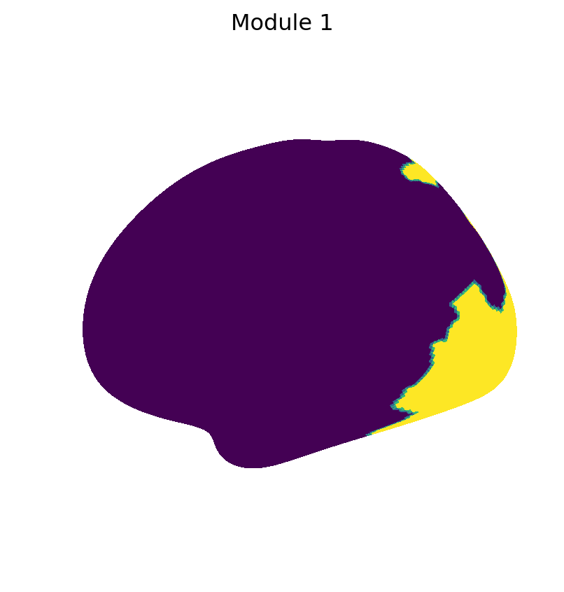
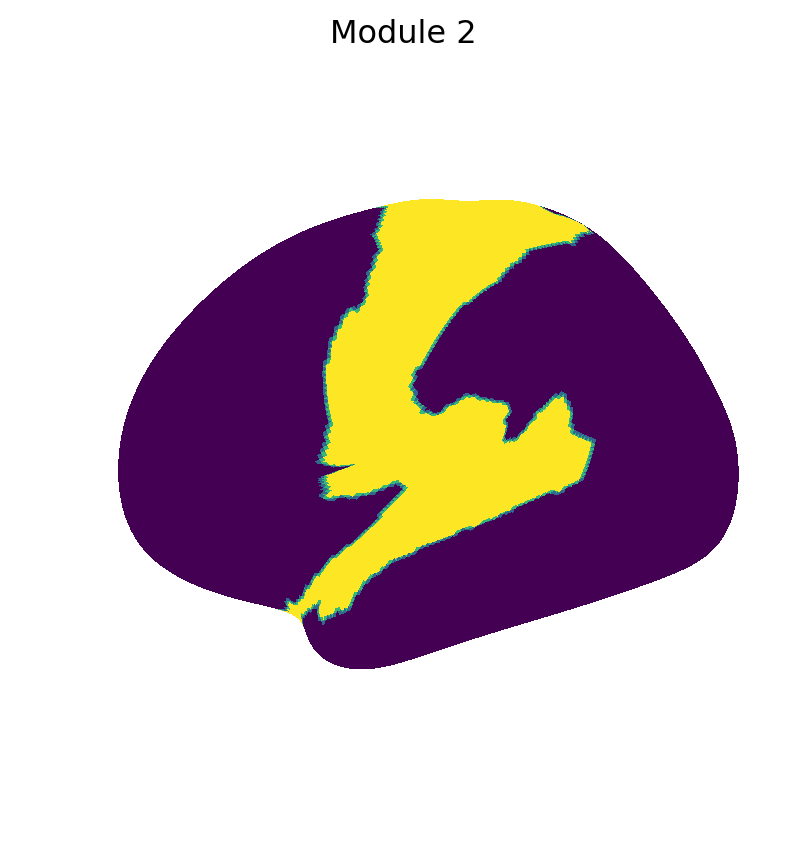
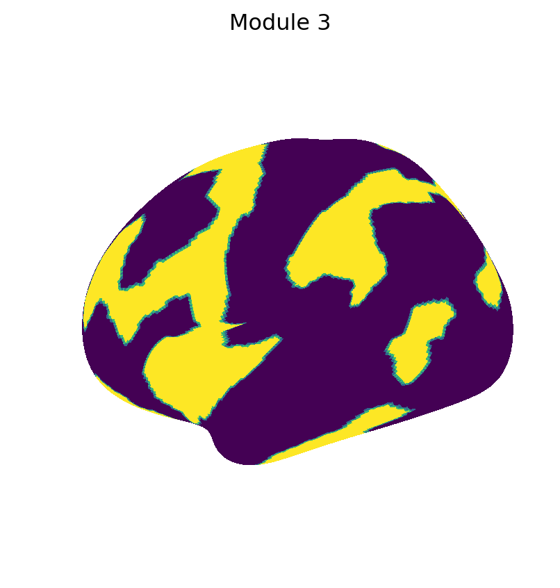
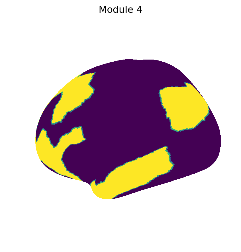
Finally, we show the maps of the individual binary m-umap embeddings.
for i inrange(M.max()+1): fig_surf(1.0* (M == i), f"Module {i+1}", "viridis")