Dispersion Centralities

Open in Colab

The squared coefficient of variation is a basic measure of normalized dispersion. It is defined as the ratio of the variance over the squared mean, or equivalently, the ratio of the first and second degrees.

Here, we show that in networks with relatively homogeneous connections within modules, the squared coefficient of variation is equivalent to a variant of the participation coefficient, a popular module-based measure of connectional diversity. It is specifically equivalent to the k-participation coefficient, the participation coefficient normalized by module size. We show these equivalences in structural and correlation co-neighbor networks from our example brain-imaging data, because these networks have high connectional homogeneity by construction.

Set up and load data

# Install abct and download abct_utils.py
base = "https://github.com/mikarubi/abct/raw/refs/heads/main"
!wget --no-clobber {base}/docs-code/examples/abct_utils.py
%pip install --quiet abct nilearn

# Import modules
import abct
import numpy as np
from abct_utils import W, C, ordw, ordc, fig_scatter, fig_surf, fig_imshow

File ‘abct_utils.py’ already there; not retrieving.

Note: you may need to restart the kernel to use updated packages.

Compute and visualize co-neighbor matrices

We first compute and visualize the co-neighbor matrices.

# Get co-neighbor matrices
Wn = abct.kneighbor(W, "common", kappa=0.1).toarray()
Cn = abct.kneighbor(C, "common", kappa=0.1).toarray()

# Visualize co-neighbor matrices
fig_imshow(Wn[np.ix_(ordw, ordw)],
          "Structural co-neighbor network",
          "inferno").show()

fig_imshow(Cn[np.ix_(ordc, ordc)],
          "Correlation co-neighbor network",
          "viridis").show()

Compute squared coefficient of variation and k-participation coefficient

We now compute the squared coefficient of variation and the k-participation coefficient for these co-neighbor networks. Note that the k-participation coefficient is defined for a specific module partition, and we therefore compute it for a range of partitions.

# Get squared coefficient of variation
WV = abct.dispersion(Wn, "coefvar2")
CV = abct.dispersion(Cn, "coefvar2")

# Get participation coefficients
K = np.arange(5, 30, 5)    # number of clusters
repl = 10                  # number of replicates

# Set random seed
np.random.seed(1)

### Run Loyvain k-modularity
WP = [None] * len(K)
CP = [None] * len(K)
for i, k in enumerate(K):
    print(f"Number of clusters: {k}")
    Mw = abct.loyvain(Wn, k, "kmodularity", replicates=repl)[0]
    Mc = abct.loyvain(Cn, k, "kmodularity", replicates=repl)[0]
    WP[i] = abct.dispersion(Wn, "kpartcoef", Mw)
    CP[i] = abct.dispersion(Cn, "kpartcoef", Mc)

Number of clusters: 5
Number of clusters: 10
Number of clusters: 15
Number of clusters: 20
Number of clusters: 25

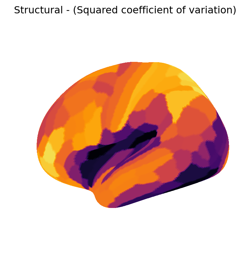
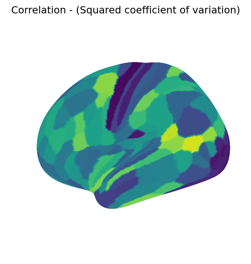
Show maps of the squared coefficient of variation

We next show the maps of the squared coefficient of variation, separately for the structural and correlation co-neighbor networks.

cv2s = {"Structural - (Squared coefficient of variation)": (- WV, "inferno"),
        "Correlation - (Squared coefficient of variation)": (- CV, "viridis")}

for i, (name, vals_cmap) in enumerate(cv2s.items()):
    vals, cmap = vals_cmap
    fig_surf(vals, name, cmap)

Scatter plots of squared coefficient of variation and k-participation coefficient

Finally, we show the scatter plots of the squared coefficient of variation and the k-participation coefficient, separately for the structural and correlation co-neighbor networks. As expected, the squared coefficient of variation and the k-participation coefficient are strongly correlated, and this correlation increases with the number of modules, as the within-module connectivity becomes more homogeneous.

normalize = lambda x: (x - x.min()) / (x.max() - x.min())

for i in range(len(K)):
    if i == 0:
        fig = fig_scatter(- np.log10(1 - WP[i]),
                            normalize(- WV))
    else:
        fig.add_scatter(x = - np.log10(1 - WP[i]),
                        y = normalize(- WV), 
                        mode="markers")

r = np.corrcoef(WV, np.array(WP))[0][1:]
fig.update_layout(xaxis_title="log-rescaled k-participation coefficient",
                  yaxis_title="rescaled - (Squared coefficient of variation)",
                  title=f"Structural network: r ~ {-np.mean(r):.3f}",
                  showlegend=False).show()

for i in range(len(K)):
    if i == 0:
        fig = fig_scatter(- np.log10(1 - CP[i]), 
                            normalize(- CV))
    else:
        fig.add_scatter(x = - np.log10(1 - CP[i]), 
                              y = normalize(- CV), 
                              mode="markers")

r = np.corrcoef(CV, np.array(CP))[0][1:]
fig.update_layout(xaxis_title="log-rescaled k-participation coefficient",
                  yaxis_title="rescaled - (Squared coefficient of variation)",
                  title=f"Correlation network: r ~ {-np.mean(r):.3f}",
                  showlegend=False).show()